Neural Thompson Sampling (NeuralTS) was introduced by Zhang et al. (2021) (Reference 1) as a way to introduce Thompson sampling (TS) to neural network prediction models. In this post, we introduce Thompson sampling, outline the problem setting for NeuralTS, describe the NeuralTS algorithm and give a bit more detail on how we can derive it.
Introduction to Thompson sampling (TS)
Thompson sampling is an algorithm for online decision problems. Imagine that we have to make a sequence of sequences across 


While we don’t know the value of 
There are many ways to use our estimate of

Greedy algorithm vs. Thompson sampling. From Russo et al. (2018). Only line 3 is different.
Contextual bandits
In the setting above (sometimes called the “context-free bandit setting”), in each round we choose an action based solely on our understanding of 

An example of the contextual bandit setting is selecting the top story to headline a news website for each user. Each request for a top story corresponds to a round, each story that could be shown represents an action, and the context vector could be features about the user (e.g. age, interests, past browsing history).
Instead of limiting the context vector to just user features, the context vector can also include arm features or features from the (user, arm) interaction.
NeuralTS
NeuralTS operates in the contextual bandit setting. Assume that we have 


Let 

Instead of sampling from the posterior distribution of 

NeuralTS algorithm (Algorithm 1 in Zhang et al.).
For completeness, 

While it might look intimidating, NeuralTS is basically using the Laplace method to approximate the output of the neural network as a Gaussian distribution with suitably chosen parameters. It maintains a Gaussian distribution for each arm’s reward. To select an arm, we sample the reward for each arm from the reward’s posterior distribution, then pull the greedy arm. Details on the Laplace method can be found in this previous post. Here are some additional notes:
- Line 1:
represents the estimated covariance matrix of
- Line 2: This is the initialization for the neural network parameters.
- Line 5: This looks like the formula for posterior variance of the target variable in the previous post but with some minor differences (it removes the additive
term but has a multiplicative
term).
- Line 6: NeuralTS adds an additional hyperparameter,
, used to control how much exploration the algorithm will do. Larger values of
.
- Line 9: In the original Laplace method, we set
to be the minimizer of a least-squares regression problem: equation (2.3) above with
. In contrast, NeuralTS takes
-regularized least-squares problem.
- Line 10: This is the posterior variance update for the neural network parameters.
References:
- Zhang, W. et al. (2021). “Neural Thompson Sampling.“
- Russo et al. (2018). A Tutorial on Thompson Sampling.
 , where
  and
and  . We have a neural network model
  which takes in an input vector
  . We would like to use the Bayesian framework to learn
  . To do that, we need to specify a prior distribution for the weights
  and precision matrix
  (inverse of covariance matrix):
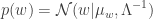
 :
:
 ‘s are fixed, our likelihood function is
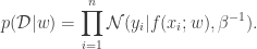

![\begin{aligned} \log p(w \mid \mathcal{D}) &= -\frac{1}{2}(w-\mu_w)^\top \Lambda (w - \mu_w) - \frac{\beta}{2}\sum_{i=1}^n \left[ f(x_i; w) - y_i \right]^2 + C \end{aligned}](https://s0.wp.com/latex.php?latex=%5Cbegin%7Baligned%7D+%5Clog+p%28w+%5Cmid+%5Cmathcal%7BD%7D%29+%26%3D+-%5Cfrac%7B1%7D%7B2%7D%28w-%5Cmu_w%29%5E%5Ctop+%5CLambda+%28w+-+%5Cmu_w%29+-+%5Cfrac%7B%5Cbeta%7D%7B2%7D%5Csum_%7Bi%3D1%7D%5En+%5Cleft%5B+f%28x_i%3B+w%29+-+y_i+%5Cright%5D%5E2+%2B+C+%5Cend%7Baligned%7D&bg=ffffff&fg=333333&s=0&c=20201002)
 . If
. If  was linear in
  has Gaussian distribution with parameters which we can derive. Unfortunately for NNs and many other prediction models,
  be the mode of the posterior
  , then we can approximate the posterior as
![\begin{aligned} \Lambda &= \left[ - \nabla^2 [\log p(w \mid \mathcal{D})] \right]_{w = w_{MAP}} \\ &= \Lambda + \frac{\beta}{2} \left[ \sum_{i=1}^n \nabla^2 \left[ f(x_i; w) - y_i \right]^2 \right]_{w = w_{MAP}}. \end{aligned}](https://s0.wp.com/latex.php?latex=%5Cbegin%7Baligned%7D+%5CLambda+%26%3D+%5Cleft%5B+-+%5Cnabla%5E2+%5B%5Clog+p%28w+%5Cmid+%5Cmathcal%7BD%7D%29%5D+%5Cright%5D_%7Bw+%3D+w_%7BMAP%7D%7D+%5C%5C++%26%3D+%5CLambda+%2B+%5Cfrac%7B%5Cbeta%7D%7B2%7D+%5Cleft%5B+%5Csum_%7Bi%3D1%7D%5En+%5Cnabla%5E2+%5Cleft%5B+f%28x_i%3B+w%29+-+y_i+%5Cright%5D%5E2+%5Cright%5D_%7Bw+%3D+w_%7BMAP%7D%7D.+%5Cend%7Baligned%7D&bg=ffffff&fg=333333&s=0&c=20201002)

 was linear in
 ![\begin{aligned} f(x; w) &\approx f(x; w_{MAP}) + g^\top (w -w_{MAP}), \\ g &= \left[ \nabla_w f(x; w) \right]_{w = w_{MAP}}. \end{aligned}](https://s0.wp.com/latex.php?latex=%5Cbegin%7Baligned%7D+f%28x%3B+w%29+%26%5Capprox+f%28x%3B+w_%7BMAP%7D%29+%2B+g%5E%5Ctop+%28w+-w_%7BMAP%7D%29%2C+%5C%5C++g+%26%3D+%5Cleft%5B+%5Cnabla_w+f%28x%3B+w%29+%5Cright%5D_%7Bw+%3D+w_%7BMAP%7D%7D.+%5Cend%7Baligned%7D&bg=ffffff&fg=333333&s=0&c=20201002)


 are the inputs,
  are the network weights,
  is the bias term for the neuron. The neuron’s output is
  .
.
 .
.
 is a parameter that is either fixed (usually at
  ) or learned from the data.
 , along with a plot of the ReLU function as the dotted line:
 when
when  , and as
  , the swish function approaches the ReLU function (it is in fact the pointwise limit). Hence, the swish function “can be loosely viewed as a smooth function which nonlinearly interpolates between the linear function and the ReLU function.”

 and
and  .
.
