In this previous post, we described how the Laplace method (or Laplace approximation) allows us to approximate a probability distribution with a Gaussian distribution with suitably chosen parameters. In this post, we show how it can be used to estimate the posterior distribution of the parameters and output of a neural network (NN), or really any prediction function. This post generally follows the exposition in Section 5.7.1 of Bishop (2006) (Reference 1).
Set-up
Assume that we are in the supervised learning setting with i.i.d. data 


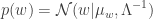
Assume the prior distribution of the network weights is normal with some mean 

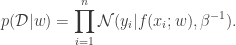
Assume that the conditional distribution of the target variable 

Since our data is i.i.d., if we assume the 
Posterior distribution of NN parameters
We now have all the ingredients we need for Bayesian inference. The posterior distribution is proportional to the product of the prior and the likelihood:

Taking logarithms on both sides:
![\begin{aligned} \log p(w \mid \mathcal{D}) &= -\frac{1}{2}(w-\mu_w)^\top \Lambda (w - \mu_w) - \frac{\beta}{2}\sum_{i=1}^n \left[ f(x_i; w) - y_i \right]^2 + C \end{aligned}](https://s0.wp.com/latex.php?latex=%5Cbegin%7Baligned%7D+%5Clog+p%28w+%5Cmid+%5Cmathcal%7BD%7D%29+%26%3D+-%5Cfrac%7B1%7D%7B2%7D%28w-%5Cmu_w%29%5E%5Ctop+%5CLambda+%28w+-+%5Cmu_w%29+-+%5Cfrac%7B%5Cbeta%7D%7B2%7D%5Csum_%7Bi%3D1%7D%5En+%5Cleft%5B+f%28x_i%3B+w%29+-+y_i+%5Cright%5D%5E2+%2B+C+%5Cend%7Baligned%7D&bg=ffffff&fg=333333&s=0&c=20201002)
for some constant 


Instead, we approximate the posterior with Laplace’s approximation. The details of Laplace’s approximation are in this previous post. we omit them here. If we let 


where
![\begin{aligned} \Lambda &= \left[ - \nabla^2 [\log p(w \mid \mathcal{D})] \right]_{w = w_{MAP}} \\ &= \Lambda + \frac{\beta}{2} \left[ \sum_{i=1}^n \nabla^2 \left[ f(x_i; w) - y_i \right]^2 \right]_{w = w_{MAP}}. \end{aligned}](https://s0.wp.com/latex.php?latex=%5Cbegin%7Baligned%7D+%5CLambda+%26%3D+%5Cleft%5B+-+%5Cnabla%5E2+%5B%5Clog+p%28w+%5Cmid+%5Cmathcal%7BD%7D%29%5D+%5Cright%5D_%7Bw+%3D+w_%7BMAP%7D%7D+%5C%5C++%26%3D+%5CLambda+%2B+%5Cfrac%7B%5Cbeta%7D%7B2%7D+%5Cleft%5B+%5Csum_%7Bi%3D1%7D%5En+%5Cnabla%5E2+%5Cleft%5B+f%28x_i%3B+w%29+-+y_i+%5Cright%5D%5E2+%5Cright%5D_%7Bw+%3D+w_%7BMAP%7D%7D.+%5Cend%7Baligned%7D&bg=ffffff&fg=333333&s=0&c=20201002)
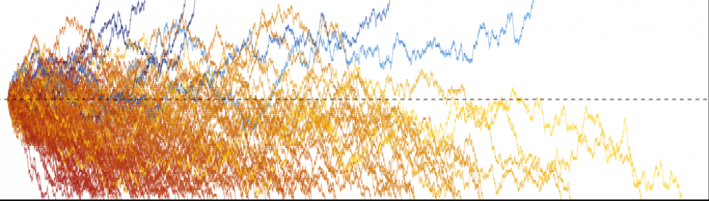
Posterior distribution of target variable
Once we have the posterior distribution of the parameters, we can get the posterior predictive distribution of the target by marginalizing out the parameters:

If the mean of 
Again we turn to a Taylor approximation to move forward. Assuming we can ignore quadratic and higher order terms,
![\begin{aligned} f(x; w) &\approx f(x; w_{MAP}) + g^\top (w -w_{MAP}), \\ g &= \left[ \nabla_w f(x; w) \right]_{w = w_{MAP}}. \end{aligned}](https://s0.wp.com/latex.php?latex=%5Cbegin%7Baligned%7D+f%28x%3B+w%29+%26%5Capprox+f%28x%3B+w_%7BMAP%7D%29+%2B+g%5E%5Ctop+%28w+-w_%7BMAP%7D%29%2C+%5C%5C++g+%26%3D+%5Cleft%5B+%5Cnabla_w+f%28x%3B+w%29+%5Cright%5D_%7Bw+%3D+w_%7BMAP%7D%7D.+%5Cend%7Baligned%7D&bg=ffffff&fg=333333&s=0&c=20201002)
With this approximation, we have a linear Gaussian model:

Applying the result for the linear Gaussian model,

References:
- Bishop, C. M. (2006). Pattern Recognition and Machine Learning (Section 4.4).

![\begin{aligned} p(y) &= \mathcal{N}\left( y \mid A\mu + b, L^{-1} + A \Lambda^{-1}A^\top \right) , \\ p(x \mid y) &= \mathcal{N} \left( x \mid \Sigma \left[ A^\top L (y - b) + \Lambda \mu \right], \Sigma \right), \end{aligned}](https://s0.wp.com/latex.php?latex=%5Cbegin%7Baligned%7D+p%28y%29+%26%3D+%5Cmathcal%7BN%7D%5Cleft%28+y+%5Cmid+A%5Cmu+%2B+b%2C+L%5E%7B-1%7D+%2B+A+%5CLambda%5E%7B-1%7DA%5E%5Ctop+%5Cright%29+%2C+%5C%5C++p%28x+%5Cmid+y%29+%26%3D+%5Cmathcal%7BN%7D+%5Cleft%28+x+%5Cmid+%5CSigma+%5Cleft%5B+A%5E%5Ctop+L+%28y+-+b%29+%2B+%5CLambda+%5Cmu+%5Cright%5D%2C+%5CSigma+%5Cright%29%2C%C2%A0%5Cend%7Baligned%7D&bg=ffffff&fg=333333&s=0&c=20201002)

 , you will find that
  is a quadratic expression in
  has Gaussian distribution. Some algebra on the expression, along with the
  follows directly from the result in
  over
over  with a Gaussian distribution
  . The approximation consists of two steps: estimating the mean
  and variance
  of the approximate Gaussian distribution.
 which maximizes
 , then the above becomes
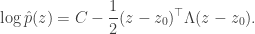
 and looking at up to the quadratic term:
![\begin{aligned} \log p(z) &\approx \log p(z_0) - \frac{1}{2}(z-z_0)^\top A (z-z_0), \\ A &= \left[ - \nabla^2 [\log p(z)] \right]_{z = z_0}. \end{aligned}](https://s0.wp.com/latex.php?latex=%5Cbegin%7Baligned%7D+%5Clog+p%28z%29+%26%5Capprox+%5Clog+p%28z_0%29+-+%5Cfrac%7B1%7D%7B2%7D%28z-z_0%29%5E%5Ctop+A+%28z-z_0%29%2C+%5C%5C++A+%26%3D+%5Cleft%5B+-+%5Cnabla%5E2+%5B%5Clog+p%28z%29%5D+%5Cright%5D_%7Bz+%3D+z_0%7D.+%5Cend%7Baligned%7D&bg=ffffff&fg=333333&s=0&c=20201002)
![[\nabla \log p(z)]_{z = z_0} = 0](https://s0.wp.com/latex.php?latex=%5B%5Cnabla+%5Clog+p%28z%29%5D_%7Bz+%3D+z_0%7D+%3D+0&bg=ffffff&fg=333333&s=0&c=20201002) . Looking at the two equations above, we see that setting
. Looking at the two equations above, we see that setting  makes the two expressions the same. This is exactly what the Laplace approximation does: it sets the precision matrix of the approximate Gaussian distribution to the Hessian of the negative log PDF of the true distribution, evaluated at the mode of the distribution.
 be the normal distribution
  on
on  be the normal distribution
  on
on ![\begin{aligned} D_{KL}(P || Q) &= \frac{1}{2}\left[ \log \frac{|\Sigma_2|}{|\Sigma_1|} - d + \text{tr}\left( \Sigma_2^{-1} \Sigma_1 \right) + (\mu_2 - \mu_1)^\top \Sigma_2^{-1} (\mu_2 - \mu_1) \right]. \end{aligned}](https://s0.wp.com/latex.php?latex=%5Cbegin%7Baligned%7D+D_%7BKL%7D%28P+%7C%7C+Q%29+%26%3D+%5Cfrac%7B1%7D%7B2%7D%5Cleft%5B+%5Clog+%5Cfrac%7B%7C%5CSigma_2%7C%7D%7B%7C%5CSigma_1%7C%7D+-+d+%2B+%5Ctext%7Btr%7D%5Cleft%28+%5CSigma_2%5E%7B-1%7D+%5CSigma_1+%5Cright%29+%2B+%28%5Cmu_2+-+%5Cmu_1%29%5E%5Ctop+%5CSigma_2%5E%7B-1%7D+%28%5Cmu_2+-+%5Cmu_1%29+%5Cright%5D.+%5Cend%7Baligned%7D&bg=ffffff&fg=333333&s=0&c=20201002)
 denote the PDF of
 ![\begin{aligned} D_{KL}(P || Q) &= \int_{\mathbb{R}^d} p(x) \log \dfrac{p(x)}{q(x)} dx \\ &= \int_{\mathbb{R}^d} \log \dfrac{|\Sigma_1|^{-1/2} \exp \left\{ -\frac{1}{2}(x-\mu_1)^\top \Sigma_1^{-1} (x - \mu_1) \right\}}{|\Sigma_2|^{-1/2} \exp \left\{ -\frac{1}{2}(x-\mu_2)^\top \Sigma_2^{-1} (x - \mu_2) \right\}} p(x) dx \\ &= \int_{\mathbb{R}^d} \left[ \frac{1}{2}\log \frac{|\Sigma_2|}{|\Sigma_1|} + \frac{1}{2}(x-\mu_2)^\top \Sigma_2^{-1} (x - \mu_2) - \frac{1}{2}(x-\mu_1)^\top \Sigma_1^{-1} (x - \mu_1) \right] p(x) dx \\ &= \frac{1}{2} \left[ \log \frac{|\Sigma_2|}{|\Sigma_1|} + \mathbb{E}_P \left[ (X-\mu_2)^\top \Sigma_2^{-1} (X - \mu_2) \right] - \mathbb{E}_P \left[ (X-\mu_1)^\top \Sigma_1^{-1} (X - \mu_1) \right] \right], \end{aligned}](https://s0.wp.com/latex.php?latex=%5Cbegin%7Baligned%7D+D_%7BKL%7D%28P+%7C%7C+Q%29+%26%3D+%5Cint_%7B%5Cmathbb%7BR%7D%5Ed%7D+p%28x%29+%5Clog+%5Cdfrac%7Bp%28x%29%7D%7Bq%28x%29%7D+dx+%5C%5C++%26%3D+%5Cint_%7B%5Cmathbb%7BR%7D%5Ed%7D%C2%A0+%5Clog+%5Cdfrac%7B%7C%5CSigma_1%7C%5E%7B-1%2F2%7D+%5Cexp+%5Cleft%5C%7B+-%5Cfrac%7B1%7D%7B2%7D%28x-%5Cmu_1%29%5E%5Ctop+%5CSigma_1%5E%7B-1%7D+%28x+-+%5Cmu_1%29+%5Cright%5C%7D%7D%7B%7C%5CSigma_2%7C%5E%7B-1%2F2%7D+%5Cexp+%5Cleft%5C%7B+-%5Cfrac%7B1%7D%7B2%7D%28x-%5Cmu_2%29%5E%5Ctop+%5CSigma_2%5E%7B-1%7D+%28x+-+%5Cmu_2%29+%5Cright%5C%7D%7D+p%28x%29+dx+%5C%5C++%26%3D+%5Cint_%7B%5Cmathbb%7BR%7D%5Ed%7D+%5Cleft%5B+%5Cfrac%7B1%7D%7B2%7D%5Clog+%5Cfrac%7B%7C%5CSigma_2%7C%7D%7B%7C%5CSigma_1%7C%7D+%2B+%5Cfrac%7B1%7D%7B2%7D%28x-%5Cmu_2%29%5E%5Ctop+%5CSigma_2%5E%7B-1%7D+%28x+-+%5Cmu_2%29+-+%5Cfrac%7B1%7D%7B2%7D%28x-%5Cmu_1%29%5E%5Ctop+%5CSigma_1%5E%7B-1%7D+%28x+-+%5Cmu_1%29+%5Cright%5D+p%28x%29+dx+%5C%5C++%26%3D+%5Cfrac%7B1%7D%7B2%7D+%5Cleft%5B+%5Clog+%5Cfrac%7B%7C%5CSigma_2%7C%7D%7B%7C%5CSigma_1%7C%7D+%2B+%5Cmathbb%7BE%7D_P+%5Cleft%5B+%28X-%5Cmu_2%29%5E%5Ctop+%5CSigma_2%5E%7B-1%7D+%28X+-+%5Cmu_2%29+%5Cright%5D+-+%5Cmathbb%7BE%7D_P+%5Cleft%5B+%28X-%5Cmu_1%29%5E%5Ctop+%5CSigma_1%5E%7B-1%7D+%28X+-+%5Cmu_1%29+%5Cright%5D+%5Cright%5D%2C+%5Cend%7Baligned%7D&bg=ffffff&fg=333333&s=0&c=20201002)
![\mathbb{E}_P[f(X)]](https://s0.wp.com/latex.php?latex=%5Cmathbb%7BE%7D_P%5Bf%28X%29%5D&bg=ffffff&fg=333333&s=0&c=20201002) denotes the expectation of
denotes the expectation of  assuming that
  . Now, we employ the trace trick to complete the proof. Using the trace trick, we know that if
  is a random vector such that
 ![\mathbb{E}[Y] = \mu](https://s0.wp.com/latex.php?latex=%5Cmathbb%7BE%7D%5BY%5D+%3D+%5Cmu&bg=ffffff&fg=333333&s=0&c=20201002) and
and  , then for any fixed matrix
  ,
,![\begin{aligned} \mathbb{E} \left[ Y^T AY \right] = \mu^T A \mu + \text{tr}(A\Sigma). \end{aligned}](https://s0.wp.com/latex.php?latex=%5Cbegin%7Baligned%7D+%5Cmathbb%7BE%7D+%5Cleft%5B+Y%5ET+AY+%5Cright%5D+%3D+%5Cmu%5ET+A+%5Cmu+%2B+%5Ctext%7Btr%7D%28A%5CSigma%29.+%5Cend%7Baligned%7D&bg=ffffff&fg=333333&s=0&c=20201002)
 with
with ![\begin{aligned} \mathbb{E}_P \left[ (X-\mu_1)^\top \Sigma_1^{-1} (X - \mu_1) \right] &= 0^\top \Sigma_1^{-1} 0 + \text{tr}(\Sigma_1^{-1} \Sigma_1) \\ &= \text{tr}(I_d) \\ &= d. \end{aligned}](https://s0.wp.com/latex.php?latex=%5Cbegin%7Baligned%7D+%5Cmathbb%7BE%7D_P+%5Cleft%5B+%28X-%5Cmu_1%29%5E%5Ctop+%5CSigma_1%5E%7B-1%7D+%28X+-+%5Cmu_1%29+%5Cright%5D+%26%3D+0%5E%5Ctop+%5CSigma_1%5E%7B-1%7D+0+%2B+%5Ctext%7Btr%7D%28%5CSigma_1%5E%7B-1%7D+%5CSigma_1%29+%5C%5C++%26%3D+%5Ctext%7Btr%7D%28I_d%29+%5C%5C++%26%3D+d.+%5Cend%7Baligned%7D&bg=ffffff&fg=333333&s=0&c=20201002)
 with
with ![\begin{aligned} \mathbb{E}_P \left[ (X-\mu_2)^\top \Sigma_2^{-1} (X - \mu_2) \right] &= (\mu_1 - \mu_2)^\top \Sigma_2^{-1} (\mu_1 - \mu_2) + \text{tr}(\Sigma_2^{-1} \Sigma_1) \\ &= (\mu_2 - \mu_1)^\top \Sigma_2^{-1} (\mu_2 - \mu_1) + \text{tr}(\Sigma_2^{-1} \Sigma_1). \end{aligned}](https://s0.wp.com/latex.php?latex=%5Cbegin%7Baligned%7D+%5Cmathbb%7BE%7D_P+%5Cleft%5B+%28X-%5Cmu_2%29%5E%5Ctop+%5CSigma_2%5E%7B-1%7D+%28X+-+%5Cmu_2%29+%5Cright%5D+%26%3D+%28%5Cmu_1+-+%5Cmu_2%29%5E%5Ctop+%5CSigma_2%5E%7B-1%7D+%28%5Cmu_1+-+%5Cmu_2%29+%2B+%5Ctext%7Btr%7D%28%5CSigma_2%5E%7B-1%7D+%5CSigma_1%29+%5C%5C++%26%3D+%28%5Cmu_2+-+%5Cmu_1%29%5E%5Ctop+%5CSigma_2%5E%7B-1%7D+%28%5Cmu_2+-+%5Cmu_1%29+%2B+%5Ctext%7Btr%7D%28%5CSigma_2%5E%7B-1%7D+%5CSigma_1%29.+%5Cend%7Baligned%7D&bg=ffffff&fg=333333&s=0&c=20201002)
 , i.e.
 ![\begin{aligned} D_{KL}(P || Q) &= \frac{1}{2}\left[ \log \frac{\sigma_2^2}{\sigma_1^2} - 1 + \frac{\sigma_1^2}{\sigma_2^2} + \frac{(\mu_2 - \mu_1)^2}{\sigma_2^2} \right] \\ &= \log \frac{\sigma_2}{\sigma_1} - \frac{1}{2} + \frac{\sigma_1^2 + (\mu_2 - \mu_1)^2}{2\sigma_2^2}, \end{aligned}](https://s0.wp.com/latex.php?latex=%5Cbegin%7Baligned%7D+D_%7BKL%7D%28P+%7C%7C+Q%29+%26%3D+%5Cfrac%7B1%7D%7B2%7D%5Cleft%5B+%5Clog+%5Cfrac%7B%5Csigma_2%5E2%7D%7B%5Csigma_1%5E2%7D+-+1+%2B+%5Cfrac%7B%5Csigma_1%5E2%7D%7B%5Csigma_2%5E2%7D+%2B+%5Cfrac%7B%28%5Cmu_2+-+%5Cmu_1%29%5E2%7D%7B%5Csigma_2%5E2%7D+%5Cright%5D+%5C%5C++%26%3D+%5Clog+%5Cfrac%7B%5Csigma_2%7D%7B%5Csigma_1%7D+-+%5Cfrac%7B1%7D%7B2%7D+%2B+%5Cfrac%7B%5Csigma_1%5E2+%2B+%28%5Cmu_2+-+%5Cmu_1%29%5E2%7D%7B2%5Csigma_2%5E2%7D%2C+%5Cend%7Baligned%7D&bg=ffffff&fg=333333&s=0&c=20201002)
 , the formula simplifies to
![\begin{aligned} D_{KL}(\mathcal{N}(\mu, \Sigma_1) || \mathcal{N}(\mu, \Sigma_2)) &= \frac{1}{2}\left[ \log \frac{|\Sigma_2|}{|\Sigma_1|} - d + \text{tr}\left( \Sigma_2^{-1} \Sigma_1 \right) \right]. \end{aligned}](https://s0.wp.com/latex.php?latex=%5Cbegin%7Baligned%7D+D_%7BKL%7D%28%5Cmathcal%7BN%7D%28%5Cmu%2C+%5CSigma_1%29+%7C%7C+%5Cmathcal%7BN%7D%28%5Cmu%2C+%5CSigma_2%29%29+%26%3D+%5Cfrac%7B1%7D%7B2%7D%5Cleft%5B+%5Clog+%5Cfrac%7B%7C%5CSigma_2%7C%7D%7B%7C%5CSigma_1%7C%7D+-+d+%2B+%5Ctext%7Btr%7D%5Cleft%28+%5CSigma_2%5E%7B-1%7D+%5CSigma_1+%5Cright%29+%5Cright%5D.+%5Cend%7Baligned%7D&bg=ffffff&fg=333333&s=0&c=20201002)
 , the formula simplifies to
![\begin{aligned} D_{KL}(\mathcal{N}(\mu_1, \Sigma) || \mathcal{N}(\mu_2, \Sigma)) &= \frac{1}{2}\left[ \log 1 - d + \text{tr}\left( I_d \right) + (\mu_2 - \mu_1)^\top \Sigma^{-1} (\mu_2 - \mu_1) \right] \\ &= \frac{1}{2}(\mu_2 - \mu_1)^\top \Sigma^{-1} (\mu_2 - \mu_1). \end{aligned}](https://s0.wp.com/latex.php?latex=%5Cbegin%7Baligned%7D+D_%7BKL%7D%28%5Cmathcal%7BN%7D%28%5Cmu_1%2C+%5CSigma%29+%7C%7C+%5Cmathcal%7BN%7D%28%5Cmu_2%2C+%5CSigma%29%29+%26%3D+%5Cfrac%7B1%7D%7B2%7D%5Cleft%5B+%5Clog+1+-+d+%2B+%5Ctext%7Btr%7D%5Cleft%28+I_d+%5Cright%29+%2B+%28%5Cmu_2+-+%5Cmu_1%29%5E%5Ctop+%5CSigma%5E%7B-1%7D+%28%5Cmu_2+-+%5Cmu_1%29+%5Cright%5D+%5C%5C++%26%3D+%5Cfrac%7B1%7D%7B2%7D%28%5Cmu_2+-+%5Cmu_1%29%5E%5Ctop+%5CSigma%5E%7B-1%7D+%28%5Cmu_2+-+%5Cmu_1%29.+%5Cend%7Baligned%7D&bg=ffffff&fg=333333&s=0&c=20201002)
 are random vectors such that
  has multivariate normal distribution:
 is invertible. Then the conditional distribution of
  given
given  is also multivariate normal, and we have explicit formulas for the conditional mean and variance:
 is the
 and the marginal distribution
  , we can plug these expressions into the formula above. After some messy algebra, we obtain the PDF of the multivariate normal with the desired parameters
  and
and  , where
  is some constant matrix with the correct dimensions that make the equation make sense. We know that
  still has multivariate normal distribution, and by standard transformation formulas we can show that
 , then the covariance between
  and
and  given
given 