In this previous post, I introduced conditional value-at-risk (CVaR), a risk measure used in mathematical finance. 


![\begin{aligned} \alpha\text{-CVaR} = \mathbb{E} \left[ X \mid X \geq q_\alpha (X) \right] .\end{aligned}](https://s0.wp.com/latex.php?latex=%5Cbegin%7Baligned%7D+%5Calpha%5Ctext%7B-CVaR%7D+%3D+%5Cmathbb%7BE%7D+%5Cleft%5B+X+%5Cmid+X+%5Cgeq+q_%5Calpha+%28X%29+%5Cright%5D+.%5Cend%7Baligned%7D&bg=ffffff&fg=333333&s=0&c=20201002)
Lemma from Rockafellar & Uryasev
It turns out that the CVaR can be thought of as the solution to a particular minimization problem. This formulation first appeared in Rockafellar & Uryasev (2000) (Reference 1), and I’ll present a simplified version here.
Denote the 


Lemma (Theorem 1 of Rockafellar & Uryasev (2000)).
satisfies
![\begin{aligned} \phi_\alpha (X) = \min_{x \in \mathbb{R}} \left[ x + \dfrac{1}{1-\alpha}\int_{-\infty}^\infty (y - x)_+ p(y) dy \right]. \end{aligned}](https://s0.wp.com/latex.php?latex=%5Cbegin%7Baligned%7D+%5Cphi_%5Calpha+%28X%29+%3D+%5Cmin_%7Bx+%5Cin+%5Cmathbb%7BR%7D%7D+%5Cleft%5B+x+%2B+%5Cdfrac%7B1%7D%7B1-%5Calpha%7D%5Cint_%7B-%5Cinfty%7D%5E%5Cinfty+%28y+-+x%29_%2B+p%28y%29+dy+%5Cright%5D.+%5Cend%7Baligned%7D&bg=ffffff&fg=333333&s=0&c=20201002)
While this lemma seems obscure, there have been applications. Reference 1 itself uses this formulation for minimizing CVaR, and see Reference 2 for a more modern application.
Where does this problem come from?
While interesting, the minimization problem seems to come out of nowhere. How does one even think to minimize such an expression as the one of the RHS?
I spent some time thinking about it and I think I have a plausible explanation. First, let’s rewrite the expression for CVaR:
![\begin{aligned} \phi_\alpha (X) &= \mathbb{E} \left[ X \mid X \geq q_\alpha (X) \right] \\ &= \dfrac{1}{\mathbb{P}\{X \geq q_\alpha (X)\}} \int_{q_\alpha(X)}^\infty y p(y) dy \\ &= \dfrac{1}{1-\alpha} \int_{q_\alpha(X)}^\infty [q_\alpha(X) + (y - q_\alpha(X))] p(y) dy \\ &= \dfrac{1}{1-\alpha}\left[ q_\alpha (X) (1-\alpha) + \int_{q_\alpha(X)}^\infty (y - q_\alpha(X)) p(y) dy \right] \\ &= q_\alpha (X) + \frac{1}{1-\alpha} \int_{-\infty}^\infty (y- q_\alpha(X))_+ p(y) dy. \end{aligned}](https://s0.wp.com/latex.php?latex=%5Cbegin%7Baligned%7D+%5Cphi_%5Calpha+%28X%29+%26%3D+%5Cmathbb%7BE%7D+%5Cleft%5B+X+%5Cmid+X+%5Cgeq+q_%5Calpha+%28X%29+%5Cright%5D+%5C%5C++%26%3D+%5Cdfrac%7B1%7D%7B%5Cmathbb%7BP%7D%5C%7BX+%5Cgeq+q_%5Calpha+%28X%29%5C%7D%7D+%5Cint_%7Bq_%5Calpha%28X%29%7D%5E%5Cinfty+y+p%28y%29+dy%C2%A0+%5C%5C++%26%3D+%5Cdfrac%7B1%7D%7B1-%5Calpha%7D+%5Cint_%7Bq_%5Calpha%28X%29%7D%5E%5Cinfty+%5Bq_%5Calpha%28X%29+%2B+%28y+-+q_%5Calpha%28X%29%29%5D+p%28y%29+dy%C2%A0+%5C%5C++%26%3D+%5Cdfrac%7B1%7D%7B1-%5Calpha%7D%5Cleft%5B+q_%5Calpha+%28X%29+%281-%5Calpha%29+%2B+%5Cint_%7Bq_%5Calpha%28X%29%7D%5E%5Cinfty+%28y+-+q_%5Calpha%28X%29%29+p%28y%29+dy+%5Cright%5D+%5C%5C++%26%3D+q_%5Calpha+%28X%29+%2B+%5Cfrac%7B1%7D%7B1-%5Calpha%7D+%5Cint_%7B-%5Cinfty%7D%5E%5Cinfty+%28y-+q_%5Calpha%28X%29%29_%2B+p%28y%29+dy.+%5Cend%7Baligned%7D&bg=ffffff&fg=333333&s=0&c=20201002)
This is exactly the RHS of the lemma, except that instead of minimizing over 

This explains why we might think about the expression on the RHS, but why should 
![\begin{aligned} q_\alpha(X) &= \underset{x \in \mathbb{R}}{\text{argmin}} \;\mathbb{E}[\rho_\alpha(X - x)]. \end{aligned}](https://s0.wp.com/latex.php?latex=%5Cbegin%7Baligned%7D+q_%5Calpha%28X%29+%26%3D+%5Cunderset%7Bx+%5Cin+%5Cmathbb%7BR%7D%7D%7B%5Ctext%7Bargmin%7D%7D+%5C%3B%5Cmathbb%7BE%7D%5B%5Crho_%5Calpha%28X+-+x%29%5D.+%5Cend%7Baligned%7D&bg=ffffff&fg=333333&s=0&c=20201002)
(This previous post presents this idea but for the empirical distribution of a sample. Note that if we define 

![\begin{aligned} \mathbb{E}[\rho_\alpha(X - x)] &= \mathbb{E}[(X - x)(\alpha - 1\{ X - x < 0 \})] \\ &= \int_{-\infty}^\infty (y - x)(\alpha - 1\{ y < x \}) p(y)dy \\ &= \int_{-\infty}^\infty (y-x)\alpha p(y) dy + \int_{-\infty}^\infty (y - x)(- 1 + 1 \{ y \geq x \}) p(y)dy \\ &= \int_{-\infty}^\infty (y-x)(\alpha-1) p(y) dy + \int_{-\infty}^\infty (y - x)1 \{ y \geq x \} p(y)dy \\ &= (\alpha-1) \mathbb{E}[X] - x(\alpha-1) + \int_{-\infty}^\infty (y-x)_+ p(y) dy \\ &= (\alpha - 1) \mathbb{E}[X] + (1 - \alpha) \left[ x + \frac{1}{1-\alpha} \int_{-\infty}^\infty (y-x)_+ p(y) dy \right] \end{aligned}](https://s0.wp.com/latex.php?latex=%5Cbegin%7Baligned%7D+%5Cmathbb%7BE%7D%5B%5Crho_%5Calpha%28X+-+x%29%5D+%26%3D+%5Cmathbb%7BE%7D%5B%28X+-+x%29%28%5Calpha+-+1%5C%7B+X+-+x+%3C+0+%5C%7D%29%5D+%5C%5C++%26%3D+%5Cint_%7B-%5Cinfty%7D%5E%5Cinfty+%28y+-+x%29%28%5Calpha+-+1%5C%7B+y+%3C+x+%5C%7D%29+p%28y%29dy+%5C%5C++%26%3D+%5Cint_%7B-%5Cinfty%7D%5E%5Cinfty+%28y-x%29%5Calpha+p%28y%29+dy+%2B+%5Cint_%7B-%5Cinfty%7D%5E%5Cinfty+%28y+-+x%29%28-+1+%2B+1+%5C%7B+y+%5Cgeq+x+%5C%7D%29+p%28y%29dy+%5C%5C++%26%3D+%5Cint_%7B-%5Cinfty%7D%5E%5Cinfty+%28y-x%29%28%5Calpha-1%29+p%28y%29+dy+%2B+%5Cint_%7B-%5Cinfty%7D%5E%5Cinfty+%28y+-+x%291+%5C%7B+y+%5Cgeq+x+%5C%7D+p%28y%29dy+%5C%5C++%26%3D+%28%5Calpha-1%29+%5Cmathbb%7BE%7D%5BX%5D+-+x%28%5Calpha-1%29+%2B+%5Cint_%7B-%5Cinfty%7D%5E%5Cinfty+%28y-x%29_%2B+p%28y%29+dy+%5C%5C++%26%3D+%28%5Calpha+-+1%29+%5Cmathbb%7BE%7D%5BX%5D+%2B+%281+-+%5Calpha%29+%5Cleft%5B+x+%2B+%5Cfrac%7B1%7D%7B1-%5Calpha%7D+%5Cint_%7B-%5Cinfty%7D%5E%5Cinfty+%28y-x%29_%2B+p%28y%29+dy+%5Cright%5D+%5Cend%7Baligned%7D&bg=ffffff&fg=333333&s=0&c=20201002)
We recognize the expression inside the square brackets as the expression we are trying to minimize over to get the
![\begin{aligned} \underset{x \in \mathbb{R}}{\text{argmin}} \;\mathbb{E}[\rho_\alpha(X - x)] &= q_\alpha(X), \\ \underset{x \in \mathbb{R}}{\min} \;\mathbb{E}[\rho_\alpha(X - x)] &= (1-\alpha) \left\{ \phi_\alpha (X) - \mathbb{E}[X] \right\}. \end{aligned}](https://s0.wp.com/latex.php?latex=%5Cbegin%7Baligned%7D+%5Cunderset%7Bx+%5Cin+%5Cmathbb%7BR%7D%7D%7B%5Ctext%7Bargmin%7D%7D+%5C%3B%5Cmathbb%7BE%7D%5B%5Crho_%5Calpha%28X+-+x%29%5D+%26%3D+q_%5Calpha%28X%29%2C+%5C%5C++%5Cunderset%7Bx+%5Cin+%5Cmathbb%7BR%7D%7D%7B%5Cmin%7D+%5C%3B%5Cmathbb%7BE%7D%5B%5Crho_%5Calpha%28X+-+x%29%5D+%26%3D%C2%A0%281-%5Calpha%29+%5Cleft%5C%7B+%5Cphi_%5Calpha+%28X%29+-+%5Cmathbb%7BE%7D%5BX%5D+%5Cright%5C%7D.+%5Cend%7Baligned%7D&bg=ffffff&fg=333333&s=0&c=20201002)
Minimizing the expression in the lemma to get the
Credit: I learnt of CVaR and this lemma through a talk that Stefan Wager gave recently at a reading group. One of his students, Roshni Sahoo, used this lemma as the basis for a new method for learning from a biased sample (see Reference 2).
References:
- Rockafellar, R. T., and Uryasev, S. (2000). “Optimization of conditional value-at-risk.“
- Sahoo, R., et al. (2022). “Learning from a Biased Sample.“
 and a level
  .
.

 of outcomes. Assuming that I’m in this set of bad outcomes, what is my expected loss?
 while investment 2 had a 0.95-CVaR of
  , which reflects our intuition that investment 2 is a riskier investment.
 , then
 and scale parameter
  , then
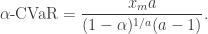
![a \in (0, 1]](https://s0.wp.com/latex.php?latex=a+%5Cin+%280%2C+1%5D&bg=ffffff&fg=333333&s=0&c=20201002) , then
, then  .)
.) and scale parameter
  , then
![\begin{aligned} \alpha\text{-CVaR} = \begin{cases} \mu + b \left( \frac{\alpha}{1-\alpha}\right) [1 - \log (2 \alpha)] &\text{if } \alpha < 1/2, \\ \mu + b \left[ 1 - \log [2(1-\alpha)] \right] &\text{if } \alpha \geq 1/2. \end{cases} \end{aligned}](https://s0.wp.com/latex.php?latex=%5Cbegin%7Baligned%7D+%5Calpha%5Ctext%7B-CVaR%7D+%3D+%5Cbegin%7Bcases%7D+%5Cmu+%2B+b+%5Cleft%28+%5Cfrac%7B%5Calpha%7D%7B1-%5Calpha%7D%5Cright%29+%5B1+-+%5Clog+%282+%5Calpha%29%5D+%26%5Ctext%7Bif+%7D+%5Calpha+%3C+1%2F2%2C+%5C%5C+%5Cmu+%2B+b+%5Cleft%5B+1+-+%5Clog+%5B2%281-%5Calpha%29%5D+%5Cright%5D+%26%5Ctext%7Bif+%7D+%5Calpha+%5Cgeq+1%2F2.+%5Cend%7Bcases%7D+%5Cend%7Baligned%7D&bg=ffffff&fg=333333&s=0&c=20201002)
 , then
 is the PDF of the standard normal distribution and
  is the
  , then
 is the
 is the binary entropy function.
 -distribution
 degrees of freedom, location parameter
 is the inverse of the standardized
  and
and  ), and
  is the PDF of the standardized
  , then
 is the