In this previous post, we defined Value at Risk (VaR): given a time horizon 

Over the time horizon
or more is
.
Why looking at VaR isn’t enough
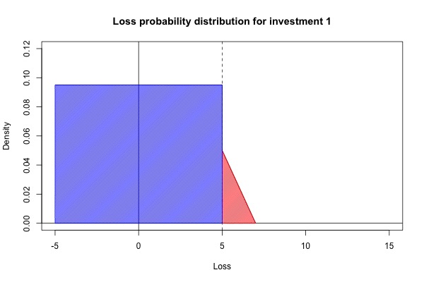
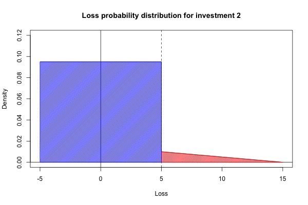
VaR helps us to understand the tail risk of the investment (in general the larger the VaR, the riskier the investment), but it doesn’t capture everything we need to know about tail risk. Consider two investments with the loss distributions shown in the figures below. Both of them have VaR at level 0.95 equal to 5. However, investment 1 can only lose up to 7% while investment 2 can lose up to 15%. In general most investors would prefer investment 1 to investment 2.
 Conditional Value at Risk (CVaR)
While VaR is unable to distinguish between the two investments above at the 95% level, conditional VaR (CVaR) is able to do so. Let’s call the tail risk a Conditional VaR at level
Let’s say I was unlucky and fell into the worst
of outcomes. Assuming that I’m in this set of bad outcomes, what is my expected loss?
In mathematical terms, CVaR is a conditional expectation: 
![\begin{aligned} \alpha\text{-CVaR} = \mathbb{E} \left[ X \mid X \geq q_\alpha (X) \right] .\end{aligned}](https://s0.wp.com/latex.php?latex=%5Cbegin%7Baligned%7D+%5Calpha%5Ctext%7B-CVaR%7D+%3D+%5Cmathbb%7BE%7D+%5Cleft%5B+X+%5Cmid+X+%5Cgeq+q_%5Calpha+%28X%29+%5Cright%5D+.%5Cend%7Baligned%7D&bg=ffffff&fg=333333&s=0&c=20201002)
In the example in the previous section, investment 1 had a 0.95-CVaR of 

CVaR for common probability distributions
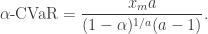
Norton et al. (2019) (Reference 3) provide formulas for some of the common probability distributions. Here are some of them (see the paper for the full list with proofs in the Appendix):
If 

If 

(If ![a \in (0, 1]](https://s0.wp.com/latex.php?latex=a+%5Cin+%280%2C+1%5D&bg=ffffff&fg=333333&s=0&c=20201002)

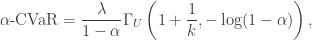
If 

![\begin{aligned} \alpha\text{-CVaR} = \begin{cases} \mu + b \left( \frac{\alpha}{1-\alpha}\right) [1 - \log (2 \alpha)] &\text{if } \alpha < 1/2, \\ \mu + b \left[ 1 - \log [2(1-\alpha)] \right] &\text{if } \alpha \geq 1/2. \end{cases} \end{aligned}](https://s0.wp.com/latex.php?latex=%5Cbegin%7Baligned%7D+%5Calpha%5Ctext%7B-CVaR%7D+%3D+%5Cbegin%7Bcases%7D+%5Cmu+%2B+b+%5Cleft%28+%5Cfrac%7B%5Calpha%7D%7B1-%5Calpha%7D%5Cright%29+%5B1+-+%5Clog+%282+%5Calpha%29%5D+%26%5Ctext%7Bif+%7D+%5Calpha+%3C+1%2F2%2C+%5C%5C+%5Cmu+%2B+b+%5Cleft%5B+1+-+%5Clog+%5B2%281-%5Calpha%29%5D+%5Cright%5D+%26%5Ctext%7Bif+%7D+%5Calpha+%5Cgeq+1%2F2.+%5Cend%7Bcases%7D+%5Cend%7Baligned%7D&bg=ffffff&fg=333333&s=0&c=20201002)
If 

where 

If 

where 
If

where 
If 


where 


If 
where 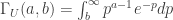
References:
- Wikipedia. Expected shortfall.
- Investopedia. Conditional Value at Risk (CVar): Definition, Uses, Formula.
- Norton, M., et al. (2019). “Calculating CVaR and bPOE for common probability distributions with application to portfolio optimization and density estimation.“

Pingback: CVaR and a lemma from Rockafellar & Uryasev | Statistical Odds & Ends