Introduction
In this previous post, we described how Quasi-Newton methods can be used to minimize a twice-differentiable function  whose domain is all of
  . At each iteration of the method, we take the following steps:
- Solve for
 in
in  .
.
- Update
 with
with 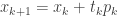 .
.
- Update
 according to some procedure.
Many methods update so that it satisfies the secant equation:

where  and
and 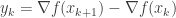 . This is often written as
  for brevity. Because this is a system of
  equations with
  unknowns, there are many ways to update .
Symmetric rank-one update (SR1)
One way to update easily is to assume that the next is the current plus a symmetric rank-one matrix, i.e.

for some  and
and  . Plugging this update into the secant equation and rearranging, we get

which implies that  must be a multiple of
  . Plugging this into the equation and solving for
  , we obtain the update
Recall from the quasi-Newton updates that we need to solve the equation  for
for  , which means that we need to compute the inverse
  to get
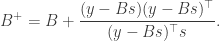
  . Because of the Sherman-Morrison-Woodbury formula, we can use the update to to derive an update for
  :
:
This is known as the SR1 update. SR1 is simple to understand and implement, but has two shortcomings. First, the denominator in the update for ,  , might be approximately zero, causing numerical issues. Second, it does not preserve positive definiteness.
References:
- Peña, J. (2016). Quasi-Newton Methods. (CMU Convex Optimization: Fall 2016, Lecture on Nov 2.)