Eigenvalues of random matrices and Wigner’s semicircle law

Random matrix theory is concerned with the study of properties of large matrices whose entries are sampled according to some known probability distribution. Usually we are interested in objects like their eigenvalues and eigenvectors.

What is interesting is that the asymptotic behavior of the random matrices is often universal, i.e. it does not depend on the probability distribution of the entries. Wigner’s semicircle law is one foundational example of that. Reference 1 goes so far to say that “the semicircle law is as important to random matrix theory as the central limit theorem is to scalar probability theory”. That’s a pretty big claim!

First, let’s define the sequence of matrices for which the semicircle law applies:

Definition (Wigner matrices): Fix  an infinite family of real-valued random variables . Define a sequence of symmetric random matrices by

Assume that:

1. The are independent.
2. The diagonal entries are identically distributed, and the off-diagonal entries are identically distributed.
3. for all .
4. (so that the off-diagonal terms are not trivially all 0 almost surely).

Then the matrices are Wigner matrices. (Sometimes, the entire sequence of matrices is referred to as a Wigner matrix.)

For , define the distribution

Wigner’s semicircle law states that if , then the limiting distribution of the eigenvalues of is . The result is stated more formally below:

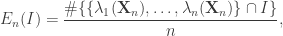
Theorem (Wigner’s semicircle law): Let be a sequence of Wigner matrices such that for all and . Let be an interval. Define the random variables

where are the eigenvalues of . Then in probability as .

(Note: Convergence in probability can be strengthened to almost sure convergence.)

See reference 2 for a proof of the semicircle law. Here, we demonstrate the semicircle law empirically. The code below generates a Wigner matrix with and computes its eigenvalues:

# make Wigner matrix and compute eigenvalues
n <- 1000
set.seed(113)
Y <- matrix(rnorm(n * n), nrow = n)
Y[lower.tri(Y)] <- 0
Y <- Y + t(Y * upper.tri(Y))
X <- Y / sqrt(n)
eigval <- eigen(X)$values

In this setting, . The code below computes the true limiting distribution and plots a histogram of the eigenvalues along with the true limit:

# truth
t <- 1
xx <- seq(-2 * sqrt(t), 2 * sqrt(t), length.out = 201)
yy <- ifelse(4 * t - xx^2 > 0, sqrt(4 * t - xx^2), 0) / (2 * pi * t)

# make plot
hist(eigval, breaks = 100, freq = FALSE, main = "Histogram of eigenvalues\nNormal(0, 1)")
lines(xx, yy, col = "red")

We can amend the code simply to have the entries have Laplace distribution (this time, we have ).

# make Wigner matrix and compute eigenvalues
n <- 1000
set.seed(113)
Y <- matrix(rexp(n * n), nrow = n) * matrix(ifelse(rnorm(n * n) > 0, 1, -1), nrow = n)
Y[lower.tri(Y)] <- 0
Y <- Y + t(Y * upper.tri(Y))
X <- Y / sqrt(n)
eigval <- eigen(X)$values

# truth
t <- 2
xx <- seq(-2 * sqrt(t), 2 * sqrt(t), length.out = 201)
yy <- ifelse(4 * t - xx^2 > 0, sqrt(4 * t - xx^2), 0) / (2 * pi * t)

# make plot
hist(eigval, breaks = 100, freq = FALSE, main = "Histogram of eigenvalues\nLaplace rate 1")
lines(xx, yy, col = "red")

What happens if the distribution of doesn’t have finite second moment? Then the theorem doesn’t hold. For example, the code below has the entries being i.i.d. Cauchy distributed (or distribution with 1 degree of freedom):

# make Wigner matrix and compute eigenvalues
n <- 1000
set.seed(113)
Y <- matrix(rt(n * n, df = 1), nrow = n)
Y[lower.tri(Y)] <- 0
Y <- Y + t(Y * upper.tri(Y))
X <- Y / sqrt(n)
eigval <- eigen(X)$values

# make plot
hist(eigval, breaks = 100, freq = FALSE, main = "Histogram of eigenvalues\nCauchy")

Notice how different the scale on the x axis is from the previous plots! Most of the eigenvalues are still within a narrow range close to 0, but there are a handful of eigenvalues that are way out. This is somewhat reminiscent of the Central Limit Theorem in scalar probability theory, where one also needs to have a finite second moment condition in order to have the desired limiting behavior.

References:

1. Feier, A. R. Methods of proof in random matrix theory.
2. Kemp, T. Math 247A: Introduction to random matrix theory.

Advertisement