logit | Statistical Odds & Ends

The logit function is defined as

$\begin{aligned} \text{logit}(p) = \log \left(\frac{p}{1-p} \right), \end{aligned}$

where $p \in (0,1)$ . The logit function transforms a variable constrained to the unit interval (usually a probability) to one that can take on any real value. In statistics, most people encounter the logit function in logistic regression, where we assume that the probability of a binary response $Y$ being 1 is associated with features $X_1, \dots, X_k$ through the relationship

$\begin{aligned} \text{logit}[\mathbb{P}(Y = 1)] = \sum_{j=1}^k \beta_j X_j. \end{aligned}$

Because the logit can take on any real value, it makes more sense to model the logit of a probability as above instead of modeling the probability directly like

$\begin{aligned} \mathbb{P}(Y = 1) = \sum_{j=1}^k \beta_j X_j. \end{aligned}$

If we model the probability directly, it is possible that $\sum_{j=1}^k \beta_j X_j$ results in a value that lies outside the unit interval; in that situation we would have to do some post-processing (e.g. thresholding) to get valid probabilities.

The expit function is simply the inverse of the logit function. It is defined as

$\begin{aligned} \text{expit}(x) = \frac{e^x}{1 + e^x}. \end{aligned}$

It takes any real number $x$ and transforms it to a value in $(0, 1)$ .

The picture below shows what the logit and expit functions look like. (Since they are inverses of each other, their graphs are reflections of each other across the $y = x$ line.)

We can think of the expit function as a special case of the softmax function. If we define the softmax function for $n$ variables as

$\begin{aligned} \sigma (x_1, \dots, x_n) = \left( \frac{e^{x_1}}{e^{x_1} + \dots + e^{x_n}}, \dots, \frac{e^{x_n}}{e^{x_1} + \dots + e^{x_n}} \right), \end{aligned}$

then when $n = 2$ ,

$\begin{aligned} \sigma(x, 0) &= \left( \frac{e^x}{e^x + e^0}, \frac{e^0}{e^x + e^0} \right) \\ &= \left( \frac{e^x}{1 + e^x}, \frac{1}{1 + e^x} \right) \\ &= \left( \text{expit}(x), 1 - \text{expit}(x) \right). \end{aligned}$

A variable $y$ is said to be ordinal if it takes on values or categories which have a natural ordering to them but the distances between the categories is not known. Ordinal variables are very common: some examples include T-shirt sizes, the Likert scale used in surveys (“for each of the following statements, choose along the scale of strongly disagree to strongly agree”), income brackets and ranked variables.

In this post, I introduce 3 commonly used methods for fitting regression models with an ordinal response. In what follows, I assume that the response variable $y$ is ordinal, taking on category values $\{ 1, 2, \dots, c \}$ . (As $y$ is ordinal, we should think of these values as category numbers instead of actual quantitative values.) We want to fit a model where we can predict $y$ based on a set of features or covariates $x \in \mathbb{R}^p$ .

Cumulative logit model with proportional odds

The cumulative logit model with proportional odds assumes the following relationship between $y$ and $x$ :

$\begin{aligned} \text{logit}[P(y \leq j)] = \log \dfrac{P(y \leq j)}{P(y > j)} = \alpha_j + \beta^T x, \qquad j = 1, \dots, c-1. \end{aligned}$

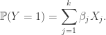
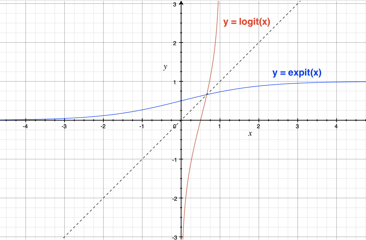
This is a natural extension of logistic regression: there, we have $c = 2$ . Note also that for fixed $j$ , the above looks like logistic regression where we have made the response binary (above $j$ vs. below or equal to $j$ ).

Note that in this model, each value of $j$ gets its own intercept $\alpha_j$ but the other coefficients $\beta$ are fixed across $j$ . Because of this, the model satisfies the proportional odds property: for all $j$ ,

$\begin{aligned} \log \left[ \dfrac{P(y \leq j \mid x_1) / P(y > j \mid x_1)}{P(y \leq j \mid x_2) / P(y > j \mid x_2)} \right] = \beta^T (x_1 - x_2). \end{aligned}$

With this model, the estimated probability of being less than or equal to $j$ is

$\begin{aligned} P(y \leq j) = \dfrac{\exp (\hat{\alpha}_j + \hat{\beta}^T x)}{1 + \exp (\hat{\alpha}_j + \hat{\beta}^T x)}. \end{aligned}$

Hence, the estimated probability of being equal to $j$ is

$\begin{aligned} P(y = j) &= P(y \leq j) - P(y \leq j - 1) \\ &= \dfrac{\exp (\hat{\alpha}_j + \hat{\beta}^T x)}{1 + \exp (\hat{\alpha}_j + \hat{\beta}^T x)} - \dfrac{\exp (\hat{\alpha}_{j-1} + \hat{\beta}^T x)}{1 + \exp (\hat{\alpha}_{j-1} + \hat{\beta}^T x)}. \end{aligned}$

Adjacent-category logit model

The adjacent-category logit model assumes the relationship

$\begin{aligned} \log \dfrac{P(y = j)}{P(y = j + 1)} = \alpha_j + \beta^T x, \qquad j = 1, \dots, c-1. \end{aligned}$

Here the odds ratio uses only adjacent categories, whereas in the cumulative logit model it uses the entire response scale. Hence, the interpretation of the model is in terms of local odds ratios as opposed to cumulative odds ratios.

Having fit the model, the estimated probability of being equal to $j$ is

$\begin{aligned} P(y = j) = \dfrac{\exp (\hat{\alpha}_j + \hat{\beta}^T x)}{1 + \sum_{k=1}^{c-1} \exp(\hat{\alpha}_k + \hat{\beta}^T x) }. \end{aligned}$

This is quite a different form from that for the cumulative logit model.

Continuation-ratio logit model

The continuation-ratio logit model assumes the relationship

$\begin{aligned} \text{logit} [P(y = j \mid y \geq j)] = \log \dfrac{P(y = j \mid y \geq j)}{P(y > j \mid y \geq j)} = \alpha_j + \beta^T x, \qquad j = 1, \dots, c-1. \end{aligned}$

Having fit the model, we have the estimated conditional probabilities

$\begin{aligned} P(Y = j \mid Y \geq j) &= \dfrac{\exp (\hat{\alpha}_j + \hat{\beta}^T x)}{1 + \exp (\hat{\alpha}_j + \hat{\beta}^T x)}. \end{aligned}$

With a bit of algebra we can convert them to unconditional probability estimates:

$\begin{aligned} P(Y = j) = \dfrac{\exp (\hat{\alpha}_j + \hat{\beta}^T x)}{1 + \exp (\hat{\alpha}_j + \hat{\beta}^T x)} \prod_{k=1}^{j-1} \dfrac{1}{1 + \exp (\hat{\alpha}_k + \hat{\beta}^T x)}. \end{aligned}$

References:

Agresti, A. (2010). Modeling Ordinal Categorical Data.

Statistical Odds & Ends

Tag Archives: logit

logit and expit

Models for ordinal responses